Development of a simulation of a lunar Lander using Deep Learning Q-Networks

The project aimed to achieve the successful landing of a lunar lander in a 2D environment by leveraging reinforcement learning and deep Q-networks.The complete code can be found in my github Page

Methodology

1. Package Import: The necessary packages and libraries were imported to support the implementation.
2. Hyperparameters: The hyperparameters for the deep Q-learning algorithm were defined, including learning rate, discount factor, exploration rate, etc.
3. Lunar Lander Environment:
   1. Action Space
   2. Observation Space
   3. Rewards
   4. Episode Termination
4. Environment Loading: The Lunar Lander environment was loaded for training and evaluation purposes.
5. Interacting with the Gym Environment: The agent interacted with the Gym environment to observe its dynamics and understand the behavior of the environment.
6. Update the Network Weights: The network weights were updated based on the loss calculated using the Bellman equation.
7. Agent Training: The agent was trained using the deep Q-learning algorithm and experience replay, gradually improving its performance over multiple episodes.
8. Trained Agent Evaluation: The trained agent was evaluated to observe its performance in the Lunar Lander environment.

Importing the Packages

numpy is a package for scientific computing in Python.

deque will be our data structure for our memory buffer.

namedtuple will be used to store the experience tuples.

The gym toolkit is a collection of environments that can be used to test reinforcement learning algorithms.

PIL.Image and pyvirtualdisplay are needed to render the Lunar Lander environment.

tensorflow.keras framework for building deep learning models.

utils is a module that contains helper functions

Hyperparameters

Hyperparameters refer to the configuration settings or parameters that define the behavior and performance of a machine learning model. Unlike model parameters, which are learned from the data during the training process, hyperparameters are set before training and remain fixed throughout the training process. They influence how the model learns and generalizes from the data.

The Hyper parameters of the lunar landing simulator is as follows:

MEMORY_SIZE = 100_000 # size of memory buffer

GAMMA = 0.995 # discount factor

ALPHA = 1e-3 # learning rate

NUM_STEPS_FOR_UPDATE = 4 # perform a learning update every C time steps

Lunar Lander Environment

An environment represents a problem or task to be solved.The goal of the Lunar Lander environment is to land the lunar lander safely on the landing pad on the surface of the moon. The landing pad is designated by two flag poles and it is always at coordinates (0,0) but the lander is also allowed to land outside of the landing pad. The lander starts at the top center of the environment with a random initial force applied to its center of mass and has infinite fuel. The environment is considered solved if the learner earns 200 points.

Action Space

The agent has four discrete actions available:

1. Do Nothing
2. Fire the right engine
3. Fire the main engine
4. Fire the left engine

Each action has a corresponding numerical value:

1. Do nothing = 0
2. Fire the right engine = 1
3. Fire the main engine = 2
4. Fire the left engine = 3

Observation Space

The agents Observation space consists of a state vector with 8 variables :

Rewards

Episode Termination

Loading the Environment

The lunar lander environment is loaded by loading the LunarLander-v2 environment from the gym library by using the .make()

env = gym.make('LunarLander-v2') #code to load the gym environment.Once we load the environment we use the reset() method to reset the environment to the initial state. The lander starts at the top center of the environment and we can render the first frame of the environment by using the .render() method.

In order to build our neural network later on we need to know the size of the state vector and the number of valid actions. We can get this information from our environment by using the .observation_space.shape and action_space.n methods, respectively.

Interacting with the Gym Environment

The Gym library implements the standard “agent-environment loop” formalism: In the standard “agent-environment loop” formalism, an agent interacts with the environment in discrete time steps 𝑡=0,1,2,.... At each time step 𝑡, the agent uses a policy 𝜋 to select an action 𝐴𝑡 based on its observation of the environment's state 𝑆𝑡. The agent receives a numerical reward 𝑅𝑡 and on the next time step, moves to a new state 𝑆𝑡+1.

Exploring the Environment's Dynamics

In Open AI's Gym environments, the .step()method is used to run a single time step of the environment's dynamics.The .step() method accepts an action and returns four values:

observation (object): an environment-specific object representing your observation of the environment. In the Lunar Lander environment this corresponds to a numpy array containing the positions and velocities of the lander

reward (float): amount of reward returned as a result of taking the given action. In the Lunar Lander environment this corresponds to a float of type numpy.float64

done (boolean): When done is True, it indicates the episode has terminated and it’s time to reset the environment.

info (dictionary): diagnostic information useful for debugging. We won't be using this variable in this notebook but it is shown here for completeness.

To begin an episode the environment has to be in the initial state this is done by using the .reset() method

Once the environment is reset, the agent can start taking actions in the environment by using the .step() method. Note that the agent can only take one action per time step. when the agent is trained a loop is used to allow the agent to take many consecutive actions during an episode.

Deep Learning Q-Network Learning

In cases where both the state and action space are discrete, we can estimate the action-value function iteratively by using the Bellman equation:

\[ Q_{i+1}(s,a) = R + \gamma \max_{a'} Q_i(s',a') \]

This iterative method converges to the optimal action-value function \( Q^*(s,a) \) as \( i \rightarrow \infty \). This means that the agent just needs to gradually explore the state-action space and keep updating the estimate of \( Q(s,a) \) until it converges to the optimal action-value function \( Q^*(s,a) \). However, in cases where the state space is continuous, it becomes practically impossible to explore the entire state-action space. Consequently, this also makes it practically impossible to gradually estimate \( Q(s,a) \) until it converges to \( Q^*(s,a) \).

In Deep Q-Learning,this problem is solved by using a neural network to estimate the action-value function \( Q(s,a) \approx Q^*(s,a) \).This neural network is called a Q-Network, and it can be trained by adjusting its weights at each iteration to minimize the mean-squared error in the Bellman equation.

Unfortunately, using neural networks in reinforcement learning to estimate action-value functions has proven to be highly unstable. Luckily, there are a couple of techniques that can be employed to avoid instabilities. These techniques consist of using a Target Network and Experience Replay.

Target Network

The Q-Network can be trained by adjusting its weights at each iteration to minimize the mean-squared error in the Bellman equation, where the target values are given by:

\( y = R + \gamma \max_{a'} Q(s', a'; w) \)

where \( w \) are the weights of the Q-Network. This means that the weights \( w \) are adjusted at each iteration to minimize the following error:

Notice that this forms a problem because the target \( y_{\text{target}} \) is changing on every iteration. To avoid oscillations and instabilities, a separate neural network is created for generating the target values.This separate neural network is called as the target Q-Network, denoted as \( \hat{Q} \), and it will have the same architecture as the original Q-Network.

By using the target Q-Network, the error becomes:

where \( w^- \) and \( w \) are the weights of the target Q-Network and the Q-Network, respectively.

In practice, the following algorithm is used : every \( C \) time step , the target Q-Network's are used to generate the target values (\( y \)) and the weights of the target Q-Network is updated by using a soft update:

\( w^- \leftarrow \tau w + (1 - \tau) w^- \)

By using the soft update, the target values are changed slowly, greatly improving the stability of the learning algorithm.

the Deep 𝑄 -Network (DQN) is a neural network that approximates the action-value function 𝑄(𝑠,𝑎)≈𝑄∗(𝑠,𝑎) . It does this by learning how to map states to 𝑄 values.

To solve the Lunar Lander environment, a DQN with the following architecture is employed:

• An Input layer that takes state_size as input.
• A Dense layer with 64 units and a ReLU activation function.
• A Dense layer with 64 units and a ReLU activation function.
• A Dense layer with num_actions units and a linear activation function. This is the output layer of the network.

This architecture allows the DQN to learn and approximate the action-value function effectively. Lastly , Adam has to be set as the optimizer with the learning rate equal to ALPHA.This was defined in the Hyperparameters section

Experience Replay

When an agent interacts with the environment, the states, actions, and rewards the agent experiences are sequential by nature. If the agent tries to learn from these consecutive experiences it can run into problems due to the strong correlations between them. To avoid this,a technique is employed known as Experience Replay to generate uncorrelated experiences for training the agent. Experience replay consists of storing the agent's experiences (i.e the states, actions, and rewards the agent receives) in a memory buffer and then sampling a random mini-batch of experiences from the buffer to do the learning. The experience tuples (𝑆𝑡,𝐴𝑡,𝑅𝑡,𝑆𝑡+1) will be added to the memory buffer at each time step as the agent interacts with the environment.

By using experience replay problematic correlations, oscillations and instabilities are avoided. In addition, experience replay also allows the agent to potentially use the same experience in multiple weight updates, which increases data efficiency.

The experience replay is combined with the Deep Q-Learning algorithm to achieve effective learning

Updating the Network's Weights

The agent_learn function is used over here. The agent_learn function will update the weights of the 𝑄 and target 𝑄̂ networks using a custom training loop. Because a custom training loop is used the gradients have to be retrived via a tf.GradientTape instance, and then call optimizer.apply_gradients() to update the weights of the 𝑄 -Network. Note that the @tf.function decorator is also used to increase performance. Without this decorator the training of the network will take twice as long.

Training the Agent

Line 1: Initialize the memory_buffer with a capacity of N = MEMORY_SIZE. Note that a deque is used as the data structure for the memory_buffer.

Line 2: Initialize the target_q_network by setting its weights equal to those of the q_network.

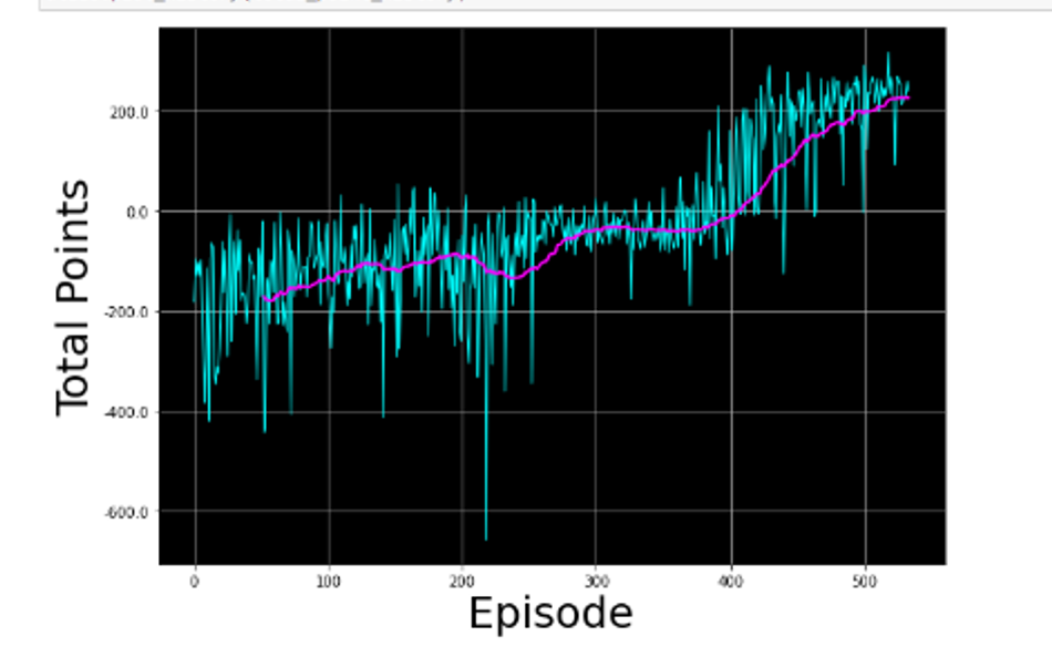
Line 3: Start the outer loop with M = num_episodes = 2000. This number is reasonable as the agent is expected to solve the Lunar Lander environment in less than 2000 episodes using the defined parameters.

Line 4: Reset the environment to the initial state and obtain the initial state.

Line 5: Start the inner loop with T = max_num_timesteps = 1000. The episode terminates automatically if it hasn't terminated after 1000 time steps.

Line 6: Observe the current state and choose an action using an ε-greedy policy. The agent starts with ε = epsilon = 1, resulting in an ε-greedy policy equivalent to the equiprobable random policy. As training progresses, decrease ε slowly towards a minimum value using a given ε-decay rate. The minimum ε value is set to 0.01 to maintain a small amount of exploration during training.

Line 7: Take the chosen action in the environment and obtain the reward and the next_state.

Line 8: Store the experience (state, action, reward, next_state, done) tuple in the memory_buffer, including the done variable to track episode termination for setting the y targets.

Line 9: Check if the conditions are met to perform a learning update using the custom ,utils.check_update_conditions function. This function verifies if C = NUM_STEPS_FOR_UPDATE = 4 time steps have occurred and if the memory_buffer has enough experience tuples to fill a mini-batch.

Lines 10 - 13: If the update variable is True, perform a learning update. This includes sampling a random mini-batch of experience tuples from the memory_buffer, setting the y targets, performing gradient descent, and updating the weights of the networks using the agent_learn function.

Line 14: Set next_state as the new state at the end of each inner loop iteration. Additionally, check if the episode has reached a terminal state (done = True) and break out of the inner loop if so.

Line 15: Update the value of ε at the end of each outer loop iteration and check if the environment has been solved. Consider the environment solved if the agent receives an average of 200 points in the last 100 episodes. If not solved, continue the outer loop and start a new episode.

Note: Additional variables are included to track the total number of points the agent received in each episode. This helps determine if the environment has been solved and provides insight into the agent's performance during training. The time module is used to measure the training duration.

The below Plot shows how the Agent improved during its training

Output

Now that the agent is trained , it can be seen in action. The utils.create_video function is used to create a video of the agent interacting with the environment using the trained 𝑄 -Network. The utils.create_video function uses the imageio library to create the video.The video of the Lunar lander landing on the landing pad can be seen in the below video

Future Scope

Reinforcement learning in robotics holds immense potential for advancing autonomous systems. By leveraging the power of reinforcement learning algorithms, robots can learn and adapt to complex environments, enabling them to perform a wide range of tasks with increased efficiency and intelligence. The integration of reinforcement learning techniques in robotics opens doors to advancements in areas such as robotic manipulation, autonomous navigation, human-robot interaction, and multi-robot systems. With further research and development, reinforcement learning has the potential to revolutionize the field of robotics, paving the way for highly capable and adaptable robotic systems that can operate in diverse real-world scenarios.

By delving into the world of reinforcement learning and mastering the concepts of Deep Q-Networks (DQN), I have unlocked a powerful tool that propels me towards becoming a proficient robotics engineer. Reinforcement learning, with its ability to train intelligent agents to make optimal decisions in dynamic environments, serves as a vital stepping stone in my journey. It has not only expanded my knowledge but also brought me closer to achieving my goals in the exciting realm of robotics.

References

Mnih, V., Kavukcuoglu, K., Silver, D. et al. Human-level control through deep reinforcement learning. Nature 518, 529–533 (2015).

Lillicrap, T. P., Hunt, J. J., Pritzel, A., et al. Continuous Control with Deep Reinforcement Learning. ICLR (2016).

Mnih, V., Kavukcuoglu, K., Silver, D. et al. Playing Atari with Deep Reinforcement Learning. arXiv e-prints. arXiv:1312.5602 (2013).